

postdoc in theory, UC Berkeley EECS & Miller Institute (off twitter, find me anywhere else)
- Tweets54
- Following378
- Followers3.9K
- Likes617




ALT Lemma 2.11 (Purifying a mixed state). There is a unitary circuit Circ(n) such that, for all mixed states ρ ∈ Cd×d of rank at most r, Circ(ρ⊗n) = E |ϱ⟩|ϱ⟩⟨ϱ|⊗n, (3) where |ϱ⟩ ∈ Cd ⊗ Cr is sampled uniformly from the space of purifications of ρ, meaning that tr2(|ϱ⟩⟨ϱ|) = ρ. Moreover, this circuit is efficient and has a gate complexity of poly(n, log(d), log(1/ε)) to perform it to ε accuracy in diamond norm distance.


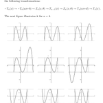
ALT Screenshot of text, transcribed here as LaTeX. "As $\theta$ traverses the interval $[-2^{n-1}, 2^{n-1}]$, Zolotarev polynomials go through the following transformations: $$-T_n(x) \to -T_n(ax + b) \to Z_n(x, \theta) \to T_{n-1}(x) \to Z_n(x, \theta) \to T_n(cx + d) \to T_n(x).$$ The next figure illustrates it for $n = 4$. [Diagram of nine different polynomials placed on a 3 by 3 grid. As one proceeds left to right, top to bottom, the polynomials appear to shift gradually, starting with an M-shaped polynomial and ending with a W-shaped one."

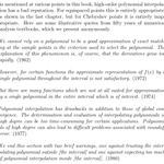
ALT The following photos are screenshots of text. That text, up to the character limit: "As mentioned at various points in this book, high-order polynomial interpola- tion has a bad reputation. For equispaced points this is entirely appropriate, as shown in the last chapter, but for Chebyshev points it is entirely inap- propriate. Here are some illustrative quotes from fifty years of numerical analysis textbooks, which we present anonymously. We cannot rely on a polynomial to be a good approximation if exact match- ing at the sample points is the criterion used to select the polynomial. The explanation of this phenomenon is, of course, that the derivatives grow too rapidly. (1962) However, for certain functions the approximate representation of f (x) by a single polynomial throughout the interval is not satisfactory. (1972) But there are many functions which are not at all suited for approximation by a single polynomial in the entire interval which is of interest. (1974)"

ALT "Although Lagrangian interpolation is sometimes useful in theoretical investi- gations, it is rarely used in practical computations. (1985) Polynomial interpolants rarely converge to a general continuous function. Polynomial interpolation is a bad idea. (1989) While theoretically important, Lagrange’s formula is, in general, not as suit- able for actual calculations as some other methods to be described below, particularly for large numbers n of support points. (1993) Unfortunately, there are functions for which interpolation at the Chebyshev points fails to converge. Moreoever, better approximations of functions like 1/(1 + x^2 ) can be obtained by other interpolants—e.g., cubic splines. (1996) In this section we consider examples which warn us of the limitations of using interpolation polynomials as approximations to functions. (1996) Increasing the number of interpolation points, i.e., increasing the degree of the polynomials, does not always lead to an improvement in the..."

ALT "The surprising state of affairs is that for most continuous functions, the quantity ||f − p_n ||_∞ will not coverge to 0. (2002) Because its derivative has n − 1 zeros, a polynomial of degree n has n − 1 extreme or inflection points. Thus, simply put, a high-degree polynomial necessarily has many “wiggles,” which may bear no relation to the data to be fit. (2002) By their very nature, polynomials of a very high degree do not constitute reasonable models for real-life phenomena, from the approximation and from the handling point-of-view. (2004) The oscillatory nature of high degree polynomials, and the property that a fluctuation over a small portion of the interval can induce large fluctuations over the entire range, restricts their use. (2005) In addition to the inherent instability of Lagrange interpolation for large n, there are also classes of functions that are not suitable for approximation by certain types of interpolation. There is a celebrated example of Runge... (2011)"

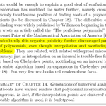
ALT "These facts would be enough to explain a good deal of confusion, but an- other consideration has muddied the water further, namely crosstalk with the notoriously troublesome problem of finding roots of a polynomial from its coefficients (to be discussed in Chapter 18). The difficulties of polyno- mial rootfinding were widely publicized by Wilkinson beginning in the 1950s, who later wrote an article called the “The perfidious polynomial” that won the Chauvenet Prize of the Mathematical Association of America [Wilkinson 1984]. Undoubtedly this negative publicity further discouraged people from the use of polynomials, even though interpolation and rootfinding are dif- ferent problems. They are related, with related widespread misconceptions about accuracy: just as interpolation on an interval is trouble-free for a stable algorithm based on Chebyshev points, rootfinding on an interval is trouble- free for a stable algorithm based on expansions in Chebyshev polynomials (Chapter 18). ..."

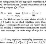
ALT screenshot of p127 of Cheney's Introduction to Approximation Theory. A rough transcription: "In order to make comparisons of the type just mentioned, we emply again the notation E_n(f) for the distance (in uniform norm) from f to the subspace of polynomials having degree <=n. Thus E_n(f) = min_{c_0,...,c_n} \max_{-1 <= x <= 1} |f(x) - \sum_{i=0}^n c_i x^i|. With this notation, the Weierstrass theorem states simply that $E_n(f) \to 0$ for all $f \in C[-1,1]$. Later on we shall establish some theorems of Jackson which state that E_n(f) converges to zero all the faster when f is smooth. At the moment we shall emply Tchebycheff expansions to establish a "lethargy" theorem: E_n(f) can converge to zero very slowly for some continuous functions. Theorem 1. If {eps_n} is any sequence converging downward to zero, then there exists an element f \in C[-1,1] such that E_n(f) >= eps_n for all n.

ALT Screenshot of the visual novel Steins;Gate of a magazine reading "SCIENCY" with a picture of Makise Kurisu on it. Text at the bottom reads "The article was about a 17-year-old girl who had just graduated from an American university. Her thesis was even published in a major scientific journal."