

Quantifying mollusks with statistical significance
Wisconsin, USA
Joined October 2023
- Tweets351
- Following350
- Followers646
- Likes1.3K





wrote up the full breakdown: poisson vs negative binomial, nfl key numbers, and why monte carlo sims depend on the distribution you pick.
bayesratings.com/blog/skewne…

Adam retweeted

Back in 2025, Pat Murphy discussed the leadership and presence Christian Yelich brings to the @Brewers 🫡
“He leads this club. He's way more important than I am. Way more important.”
#WinOurWay

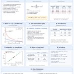
brier score is another way to grade a forecast. for each game you take the chance you gave, subtract what happened (1 if the team won, 0 if not), and square it. then average over every game. lower is better, 0 is perfect, and one game can never cost more than 1.
say you give a team 70% and they win: (0.7 − 1)² = 0.09. say you give them 90% and they lose: (0.9 − 0)² = 0.81.
calling every game 50/50 always scores 0.25, so that's the number to beat.
the useful part is that brier splits into three pieces:
- reliability: do your 70% calls actually win about 70% of the time. lower is better.
- resolution: do your forecasts move away from the average when they should. a forecaster who says 50% every game can be perfectly calibrated and still tell you nothing. higher is better.
- uncertainty: how often the team you're forecasting wins overall. it's 0.25 when wins are a 50/50 split, and it isn't up to you.
brier score = reliability − resolution + uncertainty
compared with log loss, brier is gentler on confident misses. a 90% miss costs 0.81 in brier and 2.30 in log loss. log loss cares most about the upsets you were sure wouldn't happen, and brier measures overall error. it's worth checking both.
cheat sheet below, with the live bayesratings.com scorecard for reference

log loss scores how good your probabilities were, not just whether your pick won. each game you get scored on the chance you gave the team that actually won. if you said 70% and they won, the cost is small. if you said 90% and they lost, it's big (2.30 for that one game). lower is better.
the baseline is 0.693. that's what you score by calling every game 50/50, so a forecast has to beat it to be worth anything.
calibration asks whether your percentages come true as often as you said. if you give 100 teams a 60% chance, about 60 of them should win. if only 50 do, you're overconfident.
you need both. a forecast can be calibrated but vague, or bold but wrong. log loss rewards being confident and right at the same time.
cheat sheet below, with real nfl, nhl and mlb numbers from bayesratings.com


i get so scattered when it comes to projects. i start building, get bored, and move one. to help me focus my energy, i turned my bayesian logit ratings model into a site. goal is to refine these models for each league and talk modeling sports in the blog.
bayesRatings.com


nba starts in a couple weeks and everyone loves props. i found an old project and started a rebuild. desktop app for nba props. one model per stat. set the line and compare it to the projection, then check the game log for the trend if you want.
will see how much i can get done with this, before the season starts. will need to review the models and hook up a live odds feed and maybe add in a bet tracker.
project on github. link in comment. clone, give to your coding agent, make changes to the models, add in your current odds feeds.

made some updates to sports-leader-mcp. cleaned up some processes and added get_slate tool to streamline some calls.
it makes two calls: the league scoreboard for that day, and the league injury report.
from the scoreboard it pulls each game’s eventid, start time (utc), home/away team ids and abbreviations, status and score, then consensus betting lines already on that scoreboard: american moneylines, signed homespread (negative = home favored), total, and derived no-vig win probs (home/away, plus draw for soccer).
from the injury report it attaches key out and doubtful players to each team (other statuses are just a count). it also returns a resource link to the full league injuries page.
it does not call every sportsbook. for full per-book lines, that’s still `get_game_odds`.
github.com/WalrusQuant/sport…

started working on a new trading tool for kalshi and other prediction markets. built so you can sit on a market and work both sides from one screen. the number moves, you move the quote. calling it the pit.
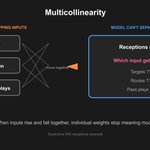
Multicollinearity
Multicollinearity is what happens when two or more inputs in a model move together so closely that the model cannot tell them apart. The overall fit can still look fine. The individual weights on each input become unstable and hard to trust.
Imagine you are modeling a WR's receptions with targets, routes run, and team pass plays. Those three often rise and fall together. If you put all of them in one model, the model may look okay overall while the weight on "targets" swings around depending on which other columns you kept. That is multicollinearity. You either drop or combine the overlapping inputs, or compress them first (PCA is one way).

Principal Component Analysis (PCA)
PCA is an important foundational tool, especially when you have lots of overlapping metrics and want to find the few underlying dimensions that actually distinguish observations. It is less a “prediction algorithm” than a way to simplify, visualize, and structure a dataset before analysis or modeling.
Imagine you have 30 golf-stat variables—driving distance, accuracy, strokes gained categories, GIR, scrambling, putting splits, etc. Many move together. PCA can compress those 30 measures into perhaps a few broad numerical dimensions, such as a mostly “ball-striking” direction and a mostly “short-game” direction, while retaining much of the variation across players.


Adam retweeted

Random Forest is an ensemble learning algorithm that combines many decision trees to produce a more stable and accurate predictor. Given training data {(xᵢ,yᵢ)}₁ⁿ, each tree is trained on a bootstrap sample of the observations, while considering a random subset of features at every split. If T₁(x),…,T_B(x) are the resulting trees, the forest prediction for regression is
f̂(x) = 1/B ∑ᵦ Tᵦ(x),
while classification typically uses majority voting. The key statistical idea is variance reduction: individual decision trees can have high variance, but averaging many sufficiently diverse trees substantially improves generalization.
Random forests are widely used in statistical machine learning because they can model complex nonlinear relationships and high-order interactions without requiring a parametric specification. They are applied to classification, regression, feature selection, anomaly detection and risk prediction. Their built-in estimates of variable importance can help identify influential predictors, while out-of-bag observations provide a convenient form of internal validation. Random forests are particularly valuable in high-dimensional problems where linear models may be too restrictive and where interpretability of a single decision tree is traded for the predictive robustness of an ensemble.

ALT Image: https://share.google/7ebtrYtHgnq18gNEs