

IOP Publishing’s Progress In series™ - an evolving network of journals that curate, enhance and amplify essential research to unite global research communities.
- Tweets526
- Following1.5K
- Followers543
- Likes541










ALT Image shows text on a light pink background. The text says: Physics World LIVE In partnership with Reports on Progress in Physics. Physics World Live: Careers. 9th April 2025, 15:00 BST - Register today


ALT Image shows a green background with a hexagon split into 6 triangles. The text on the image reads: IOP Publishing - Energy 2025 A one day event for early career researchers on the future of energy research and the green economy.

ALT Image shows text on a light pink background. The text says: Physics World LIVE In partnership with Reports on Progress in Physics. Physics World Live: Careers. 9th April 2025, 15:00 BST - Register today


ALT Image shows text on a light pink background. The text says: Physics World LIVE In partnership with Reports on Progress in Physics. Physics World Live: Careers. 9th April 2025, 15:00 BST - Register today

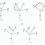
ALT Illustration taken from the open access article showing figure 2. Diagrams describing: (a) radiative corrections to the beta decay; (b) internal bremsstrahlung simultaneous to the beta decay.

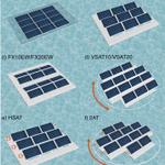
ALT Illustration taken from the open access article showing figure 5. The different FPV configurations considered. This figure is only for illustrative purposes and does not portray actual float design or panel arrangement from commercial systems.

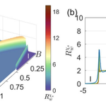
ALT Illustration taken from the open access article showing figure 10. (a) The 3D plot of the Wilson ratio R χs w maps out the phase diagram of the 1D Hubbard model at low temperatures, which significantly marks different phases of states. The parameter setting reads: T = 0.005 and u = 1. (b) A plot of the Wilson ratio R χs w at fixed B = 0.4,u = 1. As the chemical potential changes, four phases (I, II, IV and V) can be reached, indicated by sudden enhancements of the Wilson ratio.

ALT Illustration taken from the open access text showing figure 10. Constraints on axion-nucleon couplings. The laboratory constraints are from direct searches for axion-nucleon coupling and indirect searches for spin-dependent forces. Experiments at different Compton frequencies corresponds to different ALP masses ma. There are important consequences that the laboratory constraints from [58–60] exceeds the astrophysical limits. The astrophysical limits are from the analysis of [18]. Reproduced with permission from [268].

ALT Illustration taken from the open acces article showing Figure 1. Comparison between conventional-gain-based and dispersive-gain-based wireless power transfer schemes as the coupling coefficient k varies. (a) Conventional saturation-gain and dispersion-gain schemes. (b), (c) Comparison of (b) devices’ gain and (c) steady-state required gain spectrum. Circuit diagrams of the coupled resonator system using (d) parallel–parallel (PP) and (e) parallel–series (PS) topologies

ALT Image shows a light pink background with the following text in black upon it: Physics World Live - In partnership with Reports on Progress in Physics. Physics World Live: Careers 9 April 2025, 15:00 BST Register today


ALT A freshly baked apple pie with a flaky crust and a lattice design that includes the pi symbol, on a wooden table next to a cup of coffee.