
algorithmic trading
Joined July 2020
- Tweets240
- Following709
- Followers2.7K
- Likes4.4K





Yep both are almost surely 0.5 in the limit (but also I think many claimed solutions for interpretation B are bad, because they would imply that the expectation is 0.5 at finite steps, which is wrong)
Vaguely similar energy to the question 'what is the average bitcoin block interval'
If you sample a random interval, it's 10 minutes
If you sample a random point in time, the average length of the interval you land in is 20 minutes
I think it's a lot more subtle than this, and depends on the assumptions you make!
xitter.cf/GaussianProcess/status…

The answer depends on your interpretation.
Interpretation A: We sample the fraction after each child is born. Then we have a series where each element is independently boy or girl, so by symmetry the expected fraction of girls is 0.5 at each step.
Interpretation B: We sample the fraction after each family is finished. Suppose N families have finished. Then there are N girls, and some random variable B of boys. The expected fraction of girls is E[N/(N+B)] > N/(N+E[B]) = 0.5 by Jensen's inequality. So at any finite step, the expected fraction is more than 0.5! By the law of large numbers, N/(N+B) converges almost surely to 0.5 as N tends to infinity.
Interpretation C: We start with a fixed population and we want to know what happens in the long run. In fact, the population will die out, so the fraction isn't even defined. Let p be the probability that a population with one man survives. Let b_i be the probability that a man has i boys. Then p = b_0 + b_1*p + b_2*p^2+... = . The only two solutions are p=0 and p=1 (the RHS is convex, so there can be at most two). Since there is positive probability the population dies out at the first step, p != 1, so we must have p = 0.
I believe the rule is within each flashblock, you
1. Group by eoa, within each group order by nonce
2. Order groups by min(priority fee)
A similar proof, but written more combinatorially:
Pick a team of size at most pn uniformly from all possible teams. Let X_i be the indicator person i is selected.
P(X_i = 1) <= p, so we have
log(LHS) = H(X_1,…,X_n) <= H(X_1) + … + H(X_n) <= nH(p) = log(RHS)
In fact for small eps, you can do slightly better than the random construction via Reed-Solomon codes, see e.g. arxiv.org/pdf/1206.5725
So one angle for intuition here is good error correcting codes exist => you can find lots of nearly orthogonal vectors
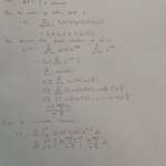
Yep, and note that your recurrence telescopes.
Another way to phrase this is to let I_k = 1 if a loop is formed when k noodles remain, and 0 otherwise. As above, E[I_k] = 1 / (2k-1).
Then by linearity of expectation,
E[loops] = E[I_100 + ... + I_1] = 1/199 + ... + 1
If you're the only arbitrageur, 1s blocks are at least as good as 2s blocks because you can replicate any 2s block performance by just ignoring every second block
As an aside, someone's feelings on short block times should match their feelings on uniform block times, because f(1)+ f(1) vs f(2) is the same comparison as f(1) + f(1) vs f(2) + f(0)
In the screenshot I'm replying to a thread where the assumed model is that MEV is proportional to sqrt(block time) xitter.cf/0xdoug/status/15657207…
In reality I think it could be convex (like in academic LVR models), ~linear (CPMM with no fee), or concave (monopolist arbitrageur)

Note that using logs in this way isn't very safe, it would be quite easy for an attacker to generate false positives, see e.g. medium.com/@naterush1997/eth…

I think mev blocker only keeps the signature private and reveals the complete unsigned tx. This stops an attacker from including a mev blocker tx in a bundle (e.g. sandwiching it), but nothing stops an attacker from sending their own competing tx, so no leak necessary here.
Yet another solution, starting from the following well known facts:
(1) If X ~ Gamma(k) and Y ~ Gamma(n), then X/(X+Y) ~ Beta(k, n) and X/(X+Y) is independent of X+Y
(2) Beta(k, n) has the same distribution as V_(k), the kth smallest of k+n-1 uniform r.v.s - (uniform r.v. order statistics)
(3) Gamma(k) ~ sum of k iid Exp(1)
(4) e^{-Exp(1)} ~ Unif(0, 1) - (probability integral transform)
(3) + (4) imply that e^-Gamma(m) ~ U_1...U_m for iid uniform U_i
(1) + (2) imply that X = (X+Y) * X/(X+Y) ~ Gamma(k+n) * V_(k)
Combining, U_1...U_k ~ (U_1...U_{k+n})^{V_(k)}
Setting k=n=1, we recover the original problem U_1 ~ (U_1U_2)^(V_1)
A nice generalization that makes what's going on clearer:
Imagine radioactive sludge decaying (i.e. a Poisson process).
Repeat the following: pick an undecayed particle i, and wait until it decays at time T_i. We retain a uniform r.v. fraction of particles at each step, so the fraction of particles undecayed after n steps is U_1...U_n.
We can also work 'backwards'. If we know that the nth particle decayed at time T_n, then we can generate T_1,...,T_{n-1} by picking n-1 uniform r.v.s V_i and setting T_i = V_(i) * T_n, where V_(i) is the ith smallest of the V_i.
If the fraction of undecayed particles at time t is k, then the fraction of undecayed particles at time ct is k^c.
Then the fraction of undecayed particles at time T_m is (U_1...U_n)^V_(m).
So we must have that (U_1....U_n)^V_(m) ~ U_1...U_m
And in particular for n=2 and m=1 we get (U_1 * U_2)^V_1 ~ U_1
As an aside, V_(m) has distribution Beta(m, n-m), and -log(U_1...U_n) has distribution Gamma(n)
So this is equivalent to Beta(m, n-m) * Gamma(n) ~ Gamma(m), a more well known fact
I addressed this in my last few sentences above.
Consider X, Y, Z which are i.i.d. uniform random variables, independent of U,V,W.
XY and UV have the same distribution and are both independent of W, so (UV)^W and (XY)^W have the same distribution, and X,Y,W are i.i.d.
Imagine a sludge of decaying radioactive particles (i.e. Poisson process).
Pick a random particle and suppose it decays at time T1. The fraction of undecayed particles is a uniform r.v. U.
Then, pick a new undecayed particle wait until decay at time T2. The fraction of undecayed particles is now UV with V uniform and independent of U.
Let W=T1/(T1+T2) be the fraction of our time we spent waiting for the first particle to decay. Then W is also uniform and is independent of UV.
Note that if there are K undecayed particles at time T, then there are K^c undecayed particles at time cT.
Then there are (UV)^W undecayed particles at time T_1, so (UV)^W = U.
Our U,V,W weren't fully independent, but U,V were independent and W was independent of UV.
So in the original setting, (XY)^Z ~ (UV)^Z ~ (UV)^W = U is still uniform.
Infinite money glitch:
If you think E[EUR per USD tomorrow] = EUR per USD today, then E[USD per EUR tomorrow] > USD per EUR today
