







Csb retweeted

yann lecun, french-american researcher born in paris in 1960, has been chief AI scientist at Meta since 2013. Meta's market cap grew from $60B to $1.5T on the back of transformers and LLMs. he spent those same years publicly telling anyone who would listen that the entire architecture was fundamentally broken.
nobody listened. the transformer became a $4.6T industry.
this october 2026 paper - independent research, not affiliated with any institution - is the mathematical proof that he was right.
standard transformers compute in a single pass. H^(l) = Attention(H^(l-1)). one shot. no persistent state. no memory between tokens. no ability to revise reasoning mid-computation.
at 1K context: transformer accuracy 40%, NCM 60%. at 8K: transformer 42%, NCM 70%. at 32K: transformer 38%, NCM 75%. at 128K tokens - the scale every enterprise deployment now requires - transformer collapses to 35%. NCM holds at 80%.
the architecture replacing it: h_{t+1} = f(h_t, x_t, θ). a continuous internal state. information doesn't pass through once and disappear. it persists. it evolves. it gets refined across multiple computation steps.
state update: h_{t+1} = h_t + Δt · F(h_t, x_t, θ). a gated continuous function. the model doesn't process the next token and move on. it updates its entire internal representation based on everything it already computed.
transformer: quadratic complexity. static weights. implicit memory. reasoning: emergent, unreliable.
NCM: linear complexity. dynamic state. explicit memory h_t. reasoning: built-in. architectural.
lecun said in 2023: "LLMs cannot reason. they cannot plan. they are not going to get us to AGI."
the research community responded by raising another $500B in LLM funding.
Meta paid him $50M+ over a decade to be the loudest critic of the technology that made them $1.4T in market cap.
in 2026, anonymous independent research notes are publishing the architecture he predicted four years ago.
the paper ends with one sentence: "NCM may not simply improve LLMs - it could mark the next generation of language models."
lecun has been writing that sentence since 2022.
save this.


Csb retweeted

Infographic by @cosmosarcive


Tensors — The Geometric Tool That Solved Einstein’s General Relativity Problem: quantamagazine.org/the-geome…
+
A book on Tensor Decompositions for Data Science [and Computational Science]: amzn.to/4s2B5g1 — extensive background materials in linear algebra, optimization, probability, & statistics are included as appendices in this book.


Csb retweeted

一套从零开始构建的通用动作捕捉系统,用于在室内自主操控多架无人机-开源
-成本只有20美金的无人机
-海外一个本科生Joshua 在他的宿舍里组装了这个无人机
-1美元的PS3 Eye摄像头,具备150fps能力
-使用了3x嵌套PID循环来实现精确控制
-代码和3D文件在github上可以查看
实现讲解:youtube.com/watch?v=0ql20JKr…
github:github.com/jyjblrd/Low-Cost-…
作者的本科论文:一套SLAM的实现:github.com/jyjblrd/distribut…
Csb retweeted

you don't even have to be in the same room
with the right Wi-Fi setup, someone walking behind brick walls can still leave a measurable trace at the receiver
the graph uses real Wallhack1.8k recordings: orange is walking, blue is an empty space, both on the same scale. the 3D scene illustrates the idea
if your next thought is “i'll just sit still,” watch the quoted post😁

breathing is enough to give you away
each breath slightly changes how Wi-Fi waves reflect off your chest. with the right receiver and processing, those tiny changes can reveal your breathing rhythm
the graphs in this animation use real WiRe-Breath recordings: orange is the rhythm extracted from Wi-Fi, gray is a reference breathing sensor
i broke down how this works, and what else you can pull out of the radio waves around you, in the article below ↓
Csb retweeted

I have been fine-tuning LLMs for over 3 years now.
Here are 5 LLM fine-tuning techniques, explained with visuals:
Traditional fine‑tuning is impractical for LLMs (billions of params; 100s of GB).
Since this kind of compute isn't accessible to everyone, parameter-efficient fine-tuning techniques (PEFT) were built.
Before we go into details of each technique, here's some background that will help you better understand these techniques:
LLM weights are matrices of numbers adjusted during fine-tuning.
Most PEFT techniques involve finding a lower-rank adaptation of these matrices, a smaller-dimensional matrix that can still represent the information stored in the original.
Now with a basic understanding of the rank of a matrix, we're in a good position to understand the different fine-tuning techniques.
(refer to the image below for a visual explanation of each technique)
1) LoRA
- Add two low-rank trainable matrices, A and B, alongside the weight matrices.
- Instead of fine-tuning W, adjust the updates in these low-rank matrices.
Even for the largest LLMs, LoRA matrices take up a few MBs of memory.
2) LoRA-FA
While LoRA significantly decreases the total trainable parameters, it requires substantial activation memory to update the low-rank weights.
LoRA-FA (FA stands for Frozen-A) freezes matrix A and only updates matrix B.
3) VeRA
- In LoRA, low-rank matrices A and B are unique for each layer.
- In VeRA, A and B are frozen, random, and shared across all layers.
- Instead, it learns layer-specific scaling VECTORS (b and d) instead.
4) Delta-LoRA
- It tunes the matrix W as well, but not in the traditional way.
- Here, the difference (or delta) between the product of matrices A and B in two consecutive training steps is added to W.
5) LoRA+
- In LoRA, both matrices A and B are updated with the same learning rate.
- Authors of LoRA+ found that setting a higher learning rate for matrix B results in better convergence.
____
Find me → @_avichawla
Every day, I share tutorials and insights on DS, ML, LLMs, and RAGs.
Csb retweeted

Check out this drone:
Joshua Bird built this drone ($20) in his dorm!
[open-source motion capture system⬇️]
Built at low cost, a motion capture system for tracking & and flying drones autonomously, with millimeter-level precision at room-scale.
The student used $1 PS3 Eye cameras with 150fps capability.
The challenge?
PID tuning! It took him 4 days of crashes to get the drone to hover, but it's still wobbly.
Used a 3x nested PID loop for precise control.
This project led to his dissertation on visual SLAM!
Full details - Algorithms for camera positioning & obstacle triangulation, in his YouTube video: youtu.be/0ql20JKrscQ
Code & 3D files on GitHub: github.com/jyjblrd/Low-Cost-…
More projects at joshuabird.com
—-
Weekly robotics and AI insights.
Subscribe free: 22Astronauts.com
Csb retweeted
Autonomous Vehicle Control: Beginner's Guide
📌 Python sample code and documentation.
This is about autonomous vehicle control algorithms. This project can be used as a technical guidebook to study the algorithms and the software architectures for beginners.
Each source code is implemented in Python to help your understanding. You can fork this repository and use it for studying, education or work freely.
📌 GitHub: github.com/ShisatoYano/Auton…
Please share if you think this could be helpful, and follow for more!
——
Weekly robotics and AI insights.
Subscribe free: 22astronauts.com
Csb retweeted

Brilliant paper by NVIDIA.
they found a way to make KV cache transferable between models.
the target model skips prefill entirely, and the conversion runs 2.7 to 25x faster than processing the context again.
let's understand why this is so important today.
LLM APIs are stateless, so every turn sends the entire conversation back to the model. the model reads it again before generating a new token, and all of it is billed as input.
prompt caching lets providers hold the KV cache for a stable prefix and bill cache hits at roughly 10% of the base input rate because that compute was already done.
this 90% reduction is one of the biggest levers in LLM serving.
but the cache only works on the model that produced it. since keys and values depend on that model's weights, another model cannot directly reuse them.
this becomes a problem with LLM routing.
if traffic moves to another model for cost or capability reasons, the accumulated KV cache becomes invalid.
the entire context must be processed again and billed at full rate.
NVIDIA's recent paper treats this as a representation problem.
prefill's main output is the KV cache, so transferring it means converting one model's cache into the representation another model expects.
they first checked whether this conversion had enough structure to exploit.
for Qwen3 14B → 32B, a linear regression from a single source layer reconstructed 56% of the variance in the target model's keys.
because models can have different layer counts, there is no natural one-to-one layer mapping.
so, for every target layer, they rank the source layers by predictive power and use the top eight together.
that pushes reconstruction to 79%.
the mapper has three parts:
> each target layer and head gets its own linear map, solved in closed form instead of with gradient descent.
> cross-layer selection chooses the source layers that best predict each target layer. their ablation shows this contributes the most.
> RoPE adds a position-dependent rotation to keys. they remove it, fit the mapping in position-free space, then apply the target model's rotation again at inference.
across six model pairs from Qwen3, Llama 3.1, and Ministral 3, four retain 73 to 98% of the receiving model's standalone accuracy.
conversion is also 3 to 25x faster than processing the context again.
prior cross-model KV reuse methods either train a neural adapter for every pair or require architecturally identical models.
this approach is closed-form and training-free, but there are still important limitations.
every tested pair belongs to the same model family, such as Qwen → Qwen or Llama → Llama.
cross-family transfer is still future work.
the tested pairs also share KV head count and per-head dimension. mismatched configurations remain untested.
and the work currently covers dense full-attention models only, not sliding-window or attention-recurrent hybrids.
link to the paper: arxiv.org/abs/2608.03893
we wrote a first-principles breakdown of how KV caching works
the article is quoted below.

Csb retweeted

🚨 TRAGEDIA EN GUAYAQUIL
El sacerdote Patricio Sánchez falleció tras caerle una cruz encima mientras celebraba una misa en la iglesia Perpetuo Socorro. El hecho conmociona a la comunidad católica. 🕊️
#Guayaquil
Cortesía
Csb retweeted

we have the technology. we just need to be brave enough to use it.
coupled 6-DOF + CFD. tail booster, four hoof jets, closed-loop landing.
Csb retweeted

ドローン空撮から3DマップとVPSマップ生成🚁
🔹メッシュ・3D Gaussian Splatting(3DGS)・点群データ(Point Cloud)の3形式で生成
🔹地上・空中のデバイス向けに、自己位置推定・ナビゲーション用のVPSマップも作成
MultiSet AIによる開発。
情報元はリプ欄。
Csb retweeted

Four rotors turn raw thrust into coordinated flight by solving a single elegant equation on the rotation group.
The vehicle’s motion is governed by
m v̇ = −τ R e₃ + m g e₃
together with the rigid-body equation
J Ω̇ + Ω × J Ω = M.
Position and velocity errors are ordinary differences; attitude error is the vee map
e_R = ½ (R_Cᵀ R − Rᵀ R_C)∨
that lives directly on SO(3).
A thrust command
τ = −(−k_x e_x − k_v e_v − m g e₃ + m ẍ_d) · R e₃
and a moment command that cancels Coriolis terms and drives both e_R and e_Ω to zero close the loop. The four motor forces are then recovered by the linear allocation matrix, so the abstract geometric commands become physical rotor speeds.
The mathematics does not approximate the sphere; it works on the sphere itself.

Csb retweeted

Each coordinate of a closed outline has its own real Fourier series: x(t) = ∑ (aₖ cos kt + bₖ sin kt), and the same for y.
A cosine and sine of frequency k make one arm of length √(aₖ² + bₖ²) turning k times per lap. One chain sets x, one sets y, and the pen sits where their guides cross. With N harmonics per axis the knight is off by 30.2 % of its height at N = 1, 0.70 % at N = 50.
At N = 1 both coordinates are pure sinusoids: an ellipse.
Csb retweeted

Osiris versus GNSS, 30 km over snow. The ground below was fully covered and the satellite map was not. Osiris matched the two anyway and touched down less than 10 m from the GNSS position, with GNSS recording only as ground truth.
Terrain in this video is masked for operational security.
Csb retweeted

pid control is one of those ideas that looks like an equation until you watch a robot actually move. imagine commanding a robotic arm to follow a trajectory. the controller constantly asks one question: where should the joint be, and where is it right now? the difference is the error. proportional control reacts to the error that exists now. large error means strong correction, small error means gentle correction. increase it too much and the robot becomes aggressive, overshoots and oscillates.
integral control remembers the past. if gravity, friction or some constant disturbance keeps leaving the joint slightly below its target, proportional control may keep producing a persistent error. the integral term accumulates that error over time and keeps increasing the correction until the bias disappears. derivative control looks in the opposite direction: it cares about how quickly the error is changing. if the robot is approaching the target too fast, derivative action pushes against that motion. think of proportional as the spring, integral as the memory, and derivative as the damper.
the interesting part is that pid is really a tiny feedback intelligence loop. observe the system, compare reality with intent, calculate the error, act, observe again. do this hundreds or thousands of times per second and a motor that knows nothing about trajectories can become a precise controlled joint. stack these loops across a robot and you begin turning electrical energy into coordinated physical behavior. before learning exotic control algorithms, understand pid deeply. it teaches the central idea behind control itself: continuously use feedback from reality to correct your model of what should happen.
